DOES DETERMINISM IMPLY CAOS IN HYDROLOGICAL VARIABLES?

¿EL DETERMINISMO IMPLICA CAOS EN VARIABLES HIDROLOGICAS?

Sebastián Marotta^(1)(2)(3)(*), Raúl Rivas ⁽¹⁾⁽³⁾, Cristian Guevara Ochoa ⁽¹⁾⁽⁴⁾ y María Florencia Degano ⁽¹⁾⁽⁴⁾

⁽¹⁾ Instituto de Hidrología de Llanuras. Azul, Buenos Aires, Argentina.

⁽²⁾ Universidad Argentina de la Empresa. Instituto de Tecnología. Buenos Aires, Argentina.

⁽³⁾ Comisión de Investigaciones Científicas de la Provincia de Buenos Aires. Buenos Aires, Argentina.

⁽⁴⁾ Consejo Nacional de Investigaciones Científicas y Técnicas. Argentina.

^(*) e_mail: smmarotta@gmail.com

ABSTRACT

In this paper we present several hydrological time series from Argentina that include, evapotranspiration, precipitation, and stream flow. We survey previous results and apply the 0-1 test for chaos to classify the sequences as regular or chaotic. Previous studies have shown evidence of chaos in several observables from hydrology using the traditional phase space reconstruction method and the computation of Lyapunov exponents. The 0-1 test for chaos can be used as a first step to identify the type of time series, that later can be subjected to the more detailed analysis of the phase space reconstruction. Assuming that the systems that generated these time series are deterministic, the 0-1 test for chaos classifies all of them as chaotic.

Keywords: Hydrology, Time series, 0-1 test for chaos, Evapotranspiration, Precipitation.

RESUMEN

En este artículo presentamos varias series de tiempo hidrológicas de Argentina que incluyen, evapotranspiración, precipitación y caudales. Revisamos previos resultados y aplicamos el test 0-1 de caos para clasificar las secuencias como regulares o caóticas. Estudios previos han demostrado evidencia de caos en muchos fenómenos hidrológicos usando el método tradicional de la reconstrucción del espacio de fase y el cálculo de exponentes de Lyapunov. El test 0-1 de caos puede ser usado como un primer paso para identificar el tipo de serie de tiempo, y que luego puede ser sujeta al análisis más detallado de la reconstrucción del espacio de fase. Si asumimos que los sistemas que generaron estas series de tiempo son determinísticos, el test 0-1 de caos las clasifica a todas ellas como caóticas.

Palabras clave: Hidrología, Series de tiempo, Test 0-1 de caos, Evapotranspiración, Precipitación.

INTRODUCTION

The hydrologic cycle is a large feedback loop that determines the conditions of water on Earth globally and locally, and with strong interactions between different systems at different spatial and temporal scales. The natural phenomena involved in the water cycle are described by physical laws and mathematical models that can explain many aspects at the microscopic and macroscopic levels, and are, in general, represented by nonlinear systems. The water cycle gathers all kinds of materials, fluids, gases, and solids, as well as organic elements with specific characteristics and properties that change with time. On the one hand, there are several external factors that have a periodic nature and are present in these systems, like the ones related to the motion of the Earth around the Sun, the rotation of the Moon around the Earth, and the rotation of the Earth about its axis, among others. These phenomena are responsible for the annual, seasonal, and daily periodic variations found in several hydrological components. On the other hand, the atmospheric agents like temperature, winds, clouds, precipitation, and the local topography and vegetation of the basins imply that the variables, like precipitation or flow discharge, are affected by many other variables in an irregular manner. These conditions represent a challenge for the meteorologist as well as for the hydrologist when trying to determine the state of a part of the system during a specific period of time. The relationship between the different interconnected systems at different scales in space and time is not completely understood.

Chaos theory gives a frame for the study of deterministic systems that present seemingly stochastic behavior and are unpredictable in the long-term. The three main ingredients of chaotic systems are, periodic behavior (regularity), sensitive dependence on initial conditions (unpredictability), and mixing (indecomposabiliy), see (Devaney, 2003). In the last few decades these properties were studied in several mathematical models, laboratory experiments and also natural phenomena, see for example, (Tsonis, 1992; Turcotte, 1997; Schreiber, 1999; Kantz and Schreiber, 2004; Sivakumar and Berndtsson, 2010; Tsonis, 2007; Skokos et al., 2016).

Several techniques have been applied to the study of hydrological time series with many different outcomes. Some researchers consider that the time series that correspond to some of these hydrological variables may be better understood when interpreted as generated by stochastic processes, and many times the predictions of stochastic models are in good agreement with the observed phenomena. For a discussion of some aspects of these interpretations see (Koutsoyiannis, 2006). Others instead, take a deterministic approach, and in some cases their predictions in the short term may be more accurate than the ones obtained with stochastic models. In 2017, Professor Sivakumar published the first book about chaos in hydrology (Sivakumar, 2017), where the different approaches are described, and the chaotic approach selected from a pragmatic point of view, with the interpretation that chaos theory can bridge the gap between stochasticity and determinism. The book is full of excellent ideas and applications, and shows the results of experiments that many researchers around the world have obtained in the study of hydrological variables. Some of the methods discussed in Sivakumar (2017) involve the phase space reconstruction, the computation of the correlation integral, the computation of Lyapunov exponents, and the study of return maps. The method of phase space reconstruction has been applied to several hydrological phenomena in the past few decades, see for example (Sivakumar, 2017; Pasternack, 1999; Sivakumar, 2000a; Sivakumar, 2002b; Sivakumar- Jayawardena, 2002; Sivakumar and Jayawardena, 2002; Sivakumar, 2004; Sivakumar and Berndtsson, 2005) and references therein.

In 2004, Gottwald and Melbourne (2004) developed a method to differentiate deterministic periodic or quasi-periodic time series from chaotic ones, using the 0-1 test for chaos. In this test, we compute a parameter K that gives a value close to 0, if the behavior of the system is regular, and a value close to 1, if the behavior is chaotic. The 0-1 test for chaos is based on sophisticated mathematics that relate group extensions and dynamics. The test was improved in the following years and has been applied to mathematical systems, laboratory measurements and also natural observables, see (Gottwald and Melbourne, 2005; Falconer et al., 2007; Gottwald and Melbourne, 2009a; Gottwald and Melbourne, 2009b; Gottwald and Melbourne, 2016). For a pedagogical overview of the mathematics behind the test see (Bernardini and Litak, 2016). In some cases, the test has also been shown to perform better than the traditional methods using phase space reconstruction and Lyapunov exponents, when the time series is contaminated with noise, see (Gottwald and Melbourne, 2016). Applications of the 0-1 test in physics, finance, and oceanography can be found in (Lugo-Fernandez, 2007; Litak et al., 2009a; Litak et al., 2009b; Krese and Goverkar, 2012; Chowdhury et al., 2012; Zachilas and Psarianos, 2012; Xin and Li, 2013; Prabin Devi et al., 2013; Krese and Govekar, 2013; Kriz and Kratochvil, 2014; Kriz, 2014). In particular, we found two applications to hydrological variables related to river flows and runoff time series in (Li et al., 2014; Kedra, 2014). Kedra (2014) used the 0-1 test and the phase space reconstruction approach.

The more traditional method of deciding if a time series is chaotic by reconstructing the phase space, finding the correlation dimension, and measuring Lyapunov exponents is very demanding in terms of computing. Each of the several steps necessary to obtain the information requires large computations and specific considerations that need careful analysis. On the other hand, the phase space reconstruction approach gives a more detailed description of the system like, for example, the minimum number of variables necessary to describe the behavior of the system in phase space. Then, the variables may be used to create a model of the system, and perform short term forecasts.

The 0-1 test has the advantage of being easy to program and work with, and takes short computation time. The test works directly with the time series and the classification is independent of the dimension of the underlying dynamical system under investigation, as well as, independent of the system being continuous (differential equations) or discrete (maps). This is a major difference with respect to the phase space reconstruction approach where the time series is considered the sample of a continuous variable, and where the dimension of the appropriate phase space of the system has to be determined in order to obtain the Lyapunov exponents to classify the system as chaotic.

As with any other test, it is necessary to use caution when applying it. Some of the problems that may arise due to oversampling continuous dynamical systems are discussed in (Melosik and Marszalek, 2016). We remark that the 0-1 test for chaos works assuming that the time series was generated by a deterministic system, and it is not relevant to test sequences generated with stochastic systems, see for example (Hu et al., 2005; Gottwald and Melbourne, 2008) for a discussion about this issue.

Methods to evaluate the evidence of chaos from a time series also require that the time series is sufficiently long to capture all aspects of the dynamics. It is not possible to assert if a natural time series of finite length has this property. For time series that may be too short to allow for convergence of K to either 0 or 1, strong indications for the behavior (regular or chaotic) can be found by looking at the values of K as a function of the length of the time series.

The application of any technique to analyze, describe, and ultimately perform forecasts depend on the characteristics of the system under study. If the system is considered stochastic, then several techniques are available for its study. When the system is considered deterministic and does not show signs of chaotic behavior, the analysis, description, and forecast (in the short and long term) are performed through modeling using differential equations. Finally, when the system is considered deterministic and shows signs of chaotic behavior, the study is of a different nature. Long term forecast is not available in these types of systems. The goal is to use the time series to reconstruct a chaotic attractor in phase space, which can provide a numerical model for the dynamics of the system and can be used for short term forecast, as seen, for example, in (Kedra, 2014). The reconstruction of the attractor is a long and difficult process that may take several months or years to perform, even when a long time series is available. Therefore, it is of great advantage to have a test, like the one described in these notes, to first classify the system as chaotic before considering such a demanding task.

In this paper we analyze several hydrological time series from Argentina that include evapotranspiration, precipitation, and stream flow. We anticipate that all of these time series are classified as chaotic by the 0-1 test. The method provides the hydrologist with a first tool for the identification of chaotic behavior that later can be refined through the use of more detailed and elaborate approaches, like for example, the phase-space reconstruction method, the computation of Lyapunov exponents, the analysis of return maps, and others.

In order to illustrate the method and compare the results, we apply the test to time series derived from the Lorenz system and the quadratic map. See Figures 1 and 2. These systems have been widely studied numerically and theoretically, and their main properties are well known, see for example, (Devaney-2003, Lorenz-1963). For the quadratic map we show one regular and one chaotic orbit.

DATA AND METHODS

Lorenz’s system.

The Lorenz system (Lorenz, 1963) is a simplified model for the phenomenon of convection in fluid dynamics. It is a continuous system of three ordinary differential equations with three parameters given by

(1)

where the dot denotes the time derivative of the variable with respect to time. The typical trajectories that are solutions of the Lorenz system are bounded and converge to a strange attractor in phase space. The solutions behave in a non-periodic fashion and the system shows sensitive dependence on initial conditions, that is, the system presents chaotic dynamics for certain values of the parameters. In particular, we use the classical values σ=10, r=28 and b=8/3. We consider the Lorenz system as a prototypical example of a continuous chaotic dynamical system with a strange attractor. Figure 1 shows the time series of the x variable and the trajectory of a solution in phase space.

The quadratic map

The quadratic family of functions f(x)=x²+µ with parameter µ, regarded as a map of the form x_n+1=x_n²+ µ, is a feedback system that presents chaotic behavior for some values of the parameter µ. It is one of the simplest nonlinear differentiable maps in one dimension, and we use it as a prototype of a discrete chaotic dynamical system, as well as, to test for a regular orbit.

Figure 2 shows two time series corresponding to regular and chaotic behavior, and the orbit diagram. The orbit diagram shows the long term behavior of a typical orbit, and the period-doubling bifurcation route to chaotic behavior characteristic of this type of map (Devaney, 2003). We can see that the value of µ =-1.3 corresponds to an attracting limiting cycle of period 4, and that a value of µ =-2 corresponds to chaotic behavior. Since theoretical results are well known for the quadratic map, we use the 0-1 test on these two sequences for illustration and comparison to the behavior of the other variables.

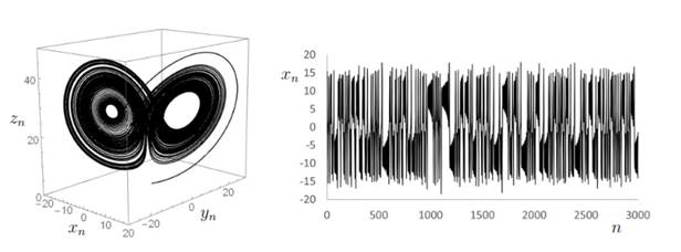
Figure 1. On the left, we see a trajectory of the Lorenz system in phase space, see equation (1). Orbits are attracted to a strange attractor, and go around two rotational centers in a non-periodic fashion. On the right, we see a chaotic time series corresponding to the variable x, for 3000 uniformly sampled points from a trajectory computed using the Runge-Kutta method of order 4 with step size 0.0001.

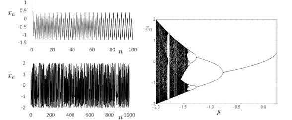
Figure 2. The quadratic family x_n+1=x_n²+µ presents different dynamical behavior for different values of the parameter µ. On the left, we see the time series of a typical orbit for µ=-1.3 (top), and µ =-2 (bottom). On the right, we see the orbit diagram for the quadratic family in the interval -2≤ µ≤ 0.25, where we see the long term behavior of typical bounded orbits. The vertical section of the diagram at µ =-1.3 shows a period-4 cycle, that corresponds to regular periodic behavior, and at µ =-2 shows chaotic behavior.

Hydrological data

The hydrological time series of evapotranspiration, precipitation, and stream flow analyzed in this paper come from the Azul and Tandil regions in the central eastern part of Argentina. See Figure 3.

The upper creek basin of Del Azul has an area of 1024 km², see (Guevara Ochoa et al., 2018), and the altitude of the basin varies between 367 and 129m. The highest part is located in the SE, in the Tandilia system and presents slopes larger than 6%, see (Poire and Spalletti, 2005). Towards the NW the basin lies in a lowland region where the slopes are smaller than 1%, see (Guevara Ochoa et al.,2019).

Figure 4 shows the hydrological time series of evapotranspiration, precipitation, and stream flows studied in this work. Table 1 presents some basic statistics of the distribution of values for the sequences including mean, standard deviation, median, skewness and kurtosis.

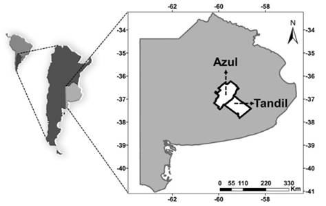
Figure 3. The picture shows, from left to right, the location of Argentina in South America, the location of the province of Buenos Aires in Argentina, and the location of Azul and Tandil areas in the province of Buenos Aires, where the hydrological variables have been measured.

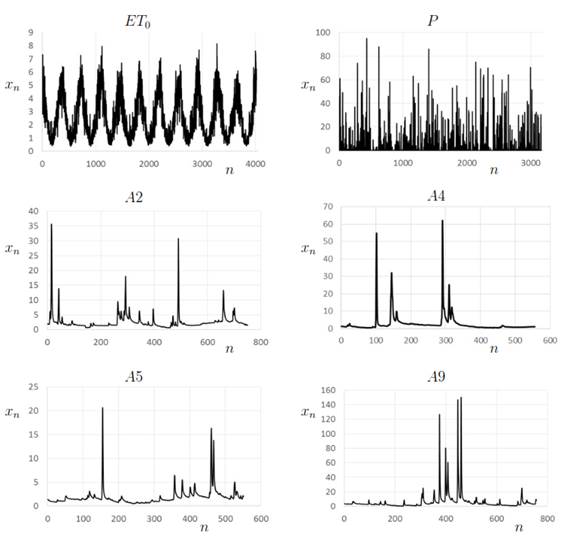
Figure 4. The time series studied in this work including evapotranspiration (ET₀), precipitation (P), and stream flows (A2, A4, A5, and A9). In these plots the horizontal axis corresponds to time in units of days.

Table 1. Basic statistical information about the time series considered in this work. Notice the large skewness characteristic of precipitation and flow time series.

Time series	Length	Mean	Std. Dev.	Median	Skewness	Kurtosis
Lorenz system	3000	-0.67	7.89	-0.98	0.15	2.35
Quadratic map with µ = -2	3000	0.00	1.41	0.02	0.00	1.50
Quadratic map with µ = -1.3	3000	-0.51	0.73	-0.62	0.08	1.14
Evapotranspiration	4018	2.67	1.62	2.33	0.51	2.20
Precipitation	3164	2.46	8.36	0.00	5.20	35.98
Stream flow A2	751	2.60	2.80	1.89	6.48	60.36
Stream flow A4	556	2.76	5.33	1.44	6.55	56.74
Stream flow A5	551	1.83	1.73	1.47	5.85	48.71
Stream flow A9	756	5.92	11.98	3.20	7.55	75.32

Evapotranspiration

Evapotranspiration is the hydrological variable of greatest relevance in the subhumid-humid Pampas, where about 85% of the water that precipitates is lost through this process, see (Weinzettel and Usunoff, 2001; Rivas et al., 2002). The estimation of the potential evapotranspiration in this area is essential, since the primary productivity is directly linked to water availability, see (Degano et al., 2018). The land use in the Azul basin is mainly rural agricultural and pastures. The highest temperatures occur during the period from December to March (summer) with a monthly average of 20°C, and the lowest temperatures occur during the period from June to August with a monthly average of 8°C.

A time series of evapotranspiration from the Tandil region is shown in Figure 4 (top left). We can see a seemingly periodic signal, but the peaks and valleys are not exactly distributed periodically in time and have different magnitudes.

Evapotranspiration from a vegetated surface depends on meteorological parameters, crop factors and environmental conditions. The process is connected to the available energy, whose main source is the direct solar radiation, and to environmental parameters such as air temperature. The driving force of this process is the difference in pressure between the water vapor on the evaporating surface and the water vapor in the surrounding atmosphere, see (Allen et al. 1998).

The Oficina de Riesgo Agropecuario (Agricultural Risk Office) calculates the Reference Evapotranspiration ET₀ with the FAO (Food and Agricultural Organization) Penman-Monteith Equation, (Allen et al., 1998), see equation (2). The ET₀ is calculated with in situ biophysical variables provided by the Sistema Meteorológico Nacional of Argentina (SMN), measured at Tandil station (n° 87645), and the data was subjected to the corresponding consistency analysis. A hypothetical reference crop with an assumed crop height of 0.12 m, a fixed surface resistance of 70 s/m, and an albedo of 0.23 were used. ET₀ is reference evapotranspiration in [mm/day], and it is given by

(2)

where R_n is the net radiation at the crop surface [MJ m^-2 day^-1], G is the soil heat flux density [MJ m^-2 day^-1], T is the mean daily air temperature at 2m height [°C], µ₂ is the wind speed at 2m height [m s^-1], e_s is the saturation vapor pressure [kPa], e_a is the actual vapor pressure [kPa], the difference e_s-e_a is the saturation vapor pressure deficit [kPa], ∆ is the slope of the vapor pressure curve [kPa °C^-1], γ is the psychrometric constant [kPa °C^-1], 0.408 is a conversion factor to mm/day, 900 is a coefficient for the reference crop [kJ^-1 Kg K day^-1], 273 is a conversion factor to express the temperature in Kelvin degrees, and 0.34 is a coefficient resulting from assuming a crop resistance of 70 s/m and an aerodynamic drag of 208/µ₂ for the reference crop [s/m].

The study of Wang et al. (Wang et al., 2014) seems to have been the first one to address evidence of chaos in an evapotranspiration time series. They applied the reconstruction method and conducted successful short term forecast experiments using local approximations obtained based on chaos theory.

Precipitation

For this study we counted with the pluviometric information from the Azul hydrometeorological station of the SMN. According to the SMN, the mean annual precipitation is 902 mm. March is the rainy month with an average precipitation of 120mm, and the months of June and July are the driest with an average of 45mm.

A time series of precipitation is shown in Figure 4 (top right). The sequence corresponds to a period of more than 8 years of measurements. The picture shows values of the daily precipitation in millimeters from a meteorological station in the Azul basin.

The precipitation time series are currently being used to reinforce the early alert system of floods in the city of Azul, see (Cazenave and Vives, 2014), and have been evaluated for several hydrometeorological studies like, for example, (Venere et al., 2004; Guevara Ochoa et al., 2017). More information about the Azul region can be found in (Barrucand et al., 2007).

Several studies of precipitation time series from the point of view of chaos theory are reviewed in (Sivakumar, 2017). Precipitation time series are often considered as the result of a stochastic process. However, this seemingly random behavior may be due to the response of a deterministic chaotic system.

Stream flow

We consider four time series of daily Azul stream flows [m³/s] denoted by A2 (751), A4 (556), A5 (551), and A9 (756), see Figure 4 and Table 1. Stream flow time series show complex behavior with a seemingly periodic base flow and peaks that corresponds to floods from irregularly distributed precipitation events. The number of variables that participate in the generation of these time series is large, but it has been found that in some cases, there are only a few generalized variables that may be able to model the behavior of the system. The study of Kedra (2014) is an excellent example of a successful application of the chaotic approach in a study of river flow. For a review of several studies of river flow using chaos theory see (Sivakumar-2017).

THE 0-1 TEST FOR CHAOS

The 0-1 test receives as input a one-dimensional time series x_n for n = 1, 2, ..., N. The data is used to drive a two-dimensional system with components given by

(3)

where c ϵ (0,2π) is a fixed constant. These new sequences, given by p_n and q_n, represent the Euclidean extensions of the system to include symmetries under rotations and translations, see (Bernardini and Litak, 2016). We are interested in the growth rate of the mean squared displacement of the trajectory (p_n, q_n) as a random walk in the plane. The starting point for the walk is set to the origin, so that p₁=q₁=0. The time-average mean squared displacement M_c(n) is given by

and its growth rate is defined by

The limits M_c(n) and K_c can be shown to exist under general conditions, and K_c takes either the value K_c =0 signifying regular dynamics, or the value K_c =1 signifying chaotic dynamics. This is justified for large classes of dynamical systems, see (Gottwald and Melbourne, 2016) and references therein. In the regular case (periodic or quasiperiodic dynamics) the trajectories for the system given by equation (3) are typically bounded, whereas in the chaotic case the trajectories typically behave like a two-dimensional Brownian motion with zero drift and hence evolve diffusively. The diffusive or bounded nature of the trajectories can be seen in a plot of the walk (p_n, q_n). A convenient method for distinguishing these growth rates, bounded or diffusive, is by means of the mean square displacement M_c(n) which accordingly is either bounded or grows linearly. The diagnostic parameter K_c captures this growth rate.

The values of M_c(n) present oscillations that sometimes make the analysis more difficult, and therefore it is convenient to adjust them before estimating the growth rate. The oscillations are computed with the following formula,

(4)

Then, the average displacement is changed from M_c(n) to D_c(n)= M_c(n)- V_c(n). When the oscillations are removed it is possible for this quantity to become negative. Then, to further set the estimator we add the term a min D_c(n) with a>1, so that the new estimator is now denoted by D_c^*(n)= D_c(n)+a min D_c(n). The value of a=1.1 is used in (Gottwald and Melbourne, 2016), as in this work.

There are several methods to measure the growth rate. The correlation method presents some advantages that have been reviewed recently in (Gottwald and Melbourne-2016), and is the one used in this work. In order to estimate the growth rate, we compute the correlation between the vectors ξ = {1, 2, 3, ..., N}, and D = {D_c^*(1), D_c^*(2), D_c^*(3), ..., D_c^*(N)} using the definition,

,

where cov and var stand for covariance and variance, respectively. The quantity K_c^* measures the level or strength of the correlation of D with a linear growth.

The final diagnostic parameter that provides the output of the test is the number K given by

(5)

where K_c^* is computed for 100 values of c chosen at random in the interval (π/5, 4π/5). This reduced interval of values of c is used to avoid resonances that can mislead the interpretation of the results. If K≈0 then the time series is classified as regular (periodic or quasi-periodic), and if K≈1 then the time series is classified as chaotic. In practice, the estimated parameter K is found for values of n<<N, and (Gottwald and Melbourne, 2016) recommends the use of N/10, as we do here.

Finally, it is convenient to plot the values of K as a function of the length of the series in order to see if there are trends, especially when it is not completely clear if the time series under analysis may be long enough to capture the full spectrum of the system dynamics.

In order to illustrate the application of the test and compare the results, we applied the test to known chaotic and regular time series from the Lorenz system and the quadratic map. See Figures 5 and 6.

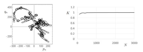
Figure 5. The 0-1 test applied to the time series of the variable x of the Lorenz system for the trajectory in Figure 1. On the left, we present a sample of the random walk of the variables p_n and q_n, given by equation (3), showing diffusive behavior. On the right, we see the parameter K given by equation (4), as a function of the length N of the time series, converging to a value of 1, and indicating chaotic motion.

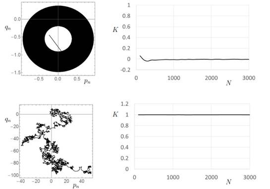
Figure 6. The 0-1 test for chaos applied to two time series from the quadratic map x_n+1=x_n+µ. At the top left, we see the random walk in the pq-plane for the case with µ =-1.3. The random walk is bounded. At the top right, we show the parameter K as a function of the length of the sequence, showing convergence to 0. The test classifies this sequence as regular, as expected. At the bottom left, we present the pq-plane showing a diffusive walk for the case µ =-2, and on the right, we see the parameter K converging to 1, as we increase the length of the sequence. The test correctly classifies this sequence as chaotic.

RESULTS

In this section we present the result of the 0-1 test for chaos, show examples of the behavior of the two dimensional walk given by the orbits of (p_n, q_n), and compute the value of K as a function of the length of the sequence, for the hydrological time series of Figure 4.

The values of K for each one of the time series is presented in Table 2, and except for the regular time series that corresponds to the periodic orbit of the quadratic function, the values of K all lie above 0.99. This means that the 0-1 test for chaos classifies the time series as chaotic.

Table 2. The results of the 0-1 test on the sequences studied in this work. The values of K in the table correspond to the median of K_c^* for 100 values of c selected at random in the interval (π/5, 4π/5), see equation (5).

Time series	K
Lorenz system	0.998
Quadratic map with µ = -2	0.998
Quadratic map with µ = -1.3	-0.006
Evapotranspiration	0.998
Precipitation	0.997
Stream flow A2	0.992
Stream flow A4	0.998
Stream flow A5	0.998
Stream flow A9	0.995

Figure 7 shows the result of the test for the time series of evapotranspiration, precipitation and stream flow studied in this work. The sample plots of an orbit of (p_n, q_n) present diffusive behavior. Moreover, in all cases, the curve of K as a function of the length of the time series shows convergence of K to 1. Even for the short time series of stream flow it is possible to see a clear trend in the behavior of K towards 1. We present the results for the sequence A9 that is representative of the behavior of the four stream flow time series.

DISCUSSION

We have presented the results of the application of the 0-1 test to several time series. For the Lorenz system and the quadratic map, the test is able to distinguish regular from chaotic behavior. For the hydrological time series of evapotranspiration, precipitation, and stream flow from Argentina, the test classified all the time series as chaotic. This implies that if we assume that these time series were generated by deterministic systems, then these systems behave chaotically. The question in the title refers to the possibility that this result applies to other hydrological observables. We also notice that with sequences of more than 500 points it is enough to have a clear idea of the convergence of the values of K.

We presented the Lorenz system as a prototype of continuous deterministic chaotic dynamics, and the quadratic equation as a prototype of discrete deterministic chaotic dynamics. We may ask if any of the systems analyzed in this work may classified in one of these two types or their several variants, i.e., is there a deterministic low dimensional nonlinear system of differential equations, like the Lorenz system, that can provide an accurate description of the dynamics? Is there a deterministic nonlinear discrete system, like the quadratic map, that could provide a good model for the description of the behavior of these variables? We can also ask if a stochastic approach would be more appropriate for some of them, and if other approaches need to be developed to understand them.

Nature seems to defy all kinds of approaches, stochastic, deterministic and chaotic. These different approaches are applied with the goal of obtaining information about different aspects of nature. However, due to the nonlinear nature of the phenomena that interact at a wide range of spatio-temporal scales, the behavior of the observables is not necessarily well represented by a superposition principle, where the sum of these characteristics gives as a result the behavior that we measure. Natural time series are the result of dynamical systems that may contain at the same time all these characteristics that we can, sometimes, get to see reflected on the results we obtain with our limited knowledge and tools.

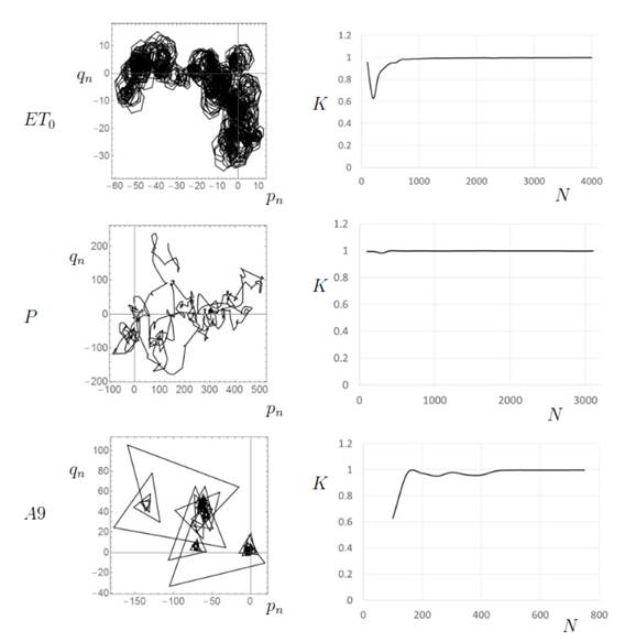
Figure 7. The result of applying the 0-1 test to time series of evapotranspiration (top), precipitation (center), and stream flow A9 (bottom). On the left, we present the random walk in the pq-plane showing diffusive behavior. On the right, we present the graphs of the parameter K as a function of the length of the time series. All sequences show convergence of K towards 1.

We stress the point suggested by the results of this paper: if we assume that the systems under study are deterministic (which not every researcher is comfortable considering as a fact), the test performed in this work classifies them as chaotic. This, in turn, implies the necessity to intensifying the study of chaotic techniques to better understand these systems in order to perform effective short term forecasts, since long term forecasts would not be possible. On the other hand, the historical problem of the availability of complete and long accurate observations is one of the main reasons that these types of study are so difficult to perform and apply.

The final answer to these types of questions remains still open, and may be considered one of the most difficult and exciting areas of research in contemporary science. Therefore, we hope that this paper provides an example, raises awareness, and underlines the use of some of the tools that are being developed and explored for a better understanding of the behavior of natural phenomena.

The results in this paper support the idea that finding evidence of chaos and performing a more detailed study of these variables may be helpful in the understanding of the dynamics of several hydrological variables, and that a first classification can be made using the 0-1 test for chaos. The study of other methods including the phase space reconstruction approach, the possible modeling of the system with local approximations, and the application of stochastic methods are left for future work.

ACKNOWLEDGEMENTES

We appreciate the Comisión de Investigaciones Científicas de la Provincia de Buenos Aires (CICPBA) and the Consejo Nacional de Investigaciones Científicas y Técnicas (CONICET), both of Argentina, for funding this research. We would like to thank Dr. Guillermo Collazos for providing us with the sequences of stream flows and for helpful discussions to improve this work. María Florencia Degano acknowledges that this work is part of her doctoral project Desarrollo e implementación de sistemas automáticos de alerta de inundaciones y sequias en el área sur de la cuenca del Rio Salado, provincia de Buenos Aires.} FONARSEC-19/13.

REFERENCES

Allen, R. G., Pereira, L. S., Raes, D., and Smith, M. (1998). Crop evapotranspiration. Guidelines for computing crop water requirements. Irrigation and Drainage Paper No. 56, FAO, Rome, Italy.

Barrucand, M. G., Vargas, W. M., Rusticucci, M. M. (2007). Dry conditions over Argentina and the related monthly circulation patterns. Meteorology and Atmospheric Physics, 98(1-2), 99-114.

Bernardini, D., Litak, G. (2016). An overview of 0-1 test for chaos. Journal of the Brazilian Society of Mechanical Sciences and Engineering, 38(5), 1433-1450.

Cazenave, G., Vives, L. (2014). Predicción de inundaciones y sistemas de alerta: Avances usando datos a tiempo real en la cuenca del arroyo del Azul. Revista de Geología Aplicada a la Ingeniería y al Ambiente, 33, 83-91.

Chowdhury, D. R., Iyengar, A. N. S., Lahiri, S. (2012). Gottwald Melbourne (0-1) test for chaos in a plasma. Nonlinear Processes in Geophysics,19, 53-56.

Degano, M. F., Rivas, E. E., Sanchez, J.M., Carmona, F., and Niclos, R. (2018). Assessment of the Potential Evapotranspiration MODIS Product Using Ground Measurements in the Pampas. To appear in Proceedings of the IEEE, ARGENCON, San Miguel de Tucuman, Tucuman, Argentina, pp. 1-5.

Devaney, R. L. (2003). An Introduction to Chaotic Dynamical Systems. Cambridge, MA, USA: Second Edition. Westview Press.

Falconer, I., Gottwald, G. A., Melbourne, I., and Wormnes, K. (2007). Application of the 0-1 Test for Chaos to Experimental Data. SIAM Journal of Applied Dynamical Systems, 6(2), 395-402.

Gottwald, G. A., Melbourne, I. (2004). A new test for chaos in deterministic systems. Proceedings of the Royal Society of London A, 460, 603-611.

Gottwald, G. A., Melbourne, I. (2005). Testing for chaos in deterministic systems with noise. Physica D, 212, 100-110.

Gottwald, G. A., Melbourne, I. (2008). Comment on ``Reliability of the 0-1 test for chaos''. Physical Review E, 77(028201), 1-3.

Gottwald, G. A., Melbourne, I. (2009a). On the Implementation of the 0-1 Test for Chaos. SIAM Journal of Applied Dynamical Systems, 8,(1), 129-145.

Gottwald, G. A., Melbourne, I. (2009b). On the validity of the 0-1 test for chaos. Nonlinearity, 22, 1367-1382.

Gottwald, G. A., Melbourne, I. (2016) The 0-1 Test for Chaos: A Review. Chapter 7. Skokos, C., Gottwald, G. A., Laskar, J. (Eds), Chaos Detection and Predictability, Lecture Notes in Physics, volume (915). Berlin, Germany: Springer-Verlag.

Guevara Ochoa, C., Briceño, N., Zimmermann, E., Vives, L., Blanco, M., Cazenave, G., Ares, G. (2017). Filling series of daily precipitation for long periods of time in plain areas. Case study superior basin of stream del Azul. Geoacta, 42(1), 38-62.

Guevara Ochoa, C., Lara, B., Vives, L., Zimmermann, E., Gandini, M. (2018). A methodology for the characterization of land use using medium-resolution spatial images. Revista Chapingo Serie Ciencias Forestales y del Ambiente, 24(2), 207-218.

Guevara Ochoa, C., Vives, L., Zimmermann, E., Masson, I., Fajardo, L., Scioli, C. (2019). Analysis and correction of digital elevation models for plain areas. Photogrammetric Engineering & Remote Sensing, 85(3), 209-219.

Hu, J., Tung, W., Gao, J., Cao, Y. (2005). Reliability of the 0-1 test for chaos. Physical Review E, 72(056207), 1-5.

Kantz, H., and Schreiber, T. (2004). Nonlinear Time Series Analysis. Cambridge, UK: Second Edition. Cambridge University Press.

Kedra, M. (2014). Deterministic chaotic dynamics of Raba River flow (Polish Carpathian Mountains). Journal of Hydrology, 509, 474-503.

Koutsoyiannis, D. (2006). On the quest for chaotic attractors in hydrological processes. Hydrological Sciences Journal, 51(6), 1065-1091.

Krese, B., Govekar, E. (2012). Nonlinear analysis of laser droplet generation by means of the 0-1 test for chaos. Nonlinear Dynamics, 67, 2101-2109.

Krese, B., Govekar, E. (2013). Analysis of traffic dynamics on a ring road-based transportation network by means of 0-1 test for chaos and Lyapunov spectrum. Transportation Research Part C, 36, 27-34.

Kriz, R. (2014). Finding Chaos in Finnish GDP. International Journal of Automation and Computing, 11(3), 231-240.

Kriz, R., Kratochvil, S. (2014). Analyses of the Chaotic Behavior of the Electricity Price Series. In Sanayei, A., Zelinka, I., Rossler, O. E., (Eds.) Interdisciplinary Symposium on Complex Systems, Emergence, Complexity and Computation, ISCS 2013, 8, 215-226. Heidelberg, Germany: Springer.

Li, X., Gao, G., Hu, T., Ma, H., Li, T.. (2014). Multiple time scales analysis of runoff series based on the Chaos Theory. Desalination and Water Treatment, 52, 2741-2749.

Litak, G., Radons, G., Schubert, S. (2009a). Identification of chaos in a regenerative cutting process by the 0-1 test. Proceedings in Applied Mathematics and Mechanics, 9, 299-300.

Litak, G., Syta, A., Wiercigroch. M. (2009b). Identification of chaos in a cutting process by the 0-1 test. Chaos, Solitons and Fractals, 40, 2095-2101.

Lorenz, E. N. (1963). Deterministic Nonperiodic Flow. Journal of the Atmospheric Sciences, 20(2), 130-141.

Lugo-Fernandez, A. (2007). Is the Loop Current a Chaotic Oscillator? Journal of Physical Oceanography, 37, 1455-1469.

Melosik, M., Marszalek, W. (2016). On the 0/1 test for chaos in continuous systems. Bulletin of the Polish Academy of Sciences, Technical Sciences, 64(3),521-528.

Pasternack, G. B. (1999). Does the river run wild? Assessing chaos in hydrological systems. Elsevier Advances in Water Resources, 23, 253-260.

Prabin Devi1, S., Singh, S. B., Surjalal Sharma, A. (2013). Deterministic dynamics of the magnetosphere: results of the 0-1 test. Nonlinear Processes in Geophysics, 20, 11-18.

Poire, D. G., Spalletti, L. A. (2005). La cubierta sedimentaria precámbrica/paleozoica inferior del Sistema de Tandilia. In De Barrio, R. E., Etcheverry, R. O., Caballe, M. F., Llambias, E. (Eds.), Geología y Recursos Minerales de la provincia de Buenos Aires. Relatorio del XVI Congreso Geológico Argentino, pp. 51-68.

Rivas, R., Caselles, V., and Usunoff, E. (2002). Reference evapotranspiration in the Azul River Basin, Argentina. In Bocanegra, E., Martinez, D., y Massone, H. (Eds.), Actas XXXII AIH & VI ALHSUD Congress of Groundwater and Human Development, Mar del Plata, Argentina, pp. 693-700.

Schreiber, T. (1999). Interdisciplinary application of nonlinear time series methods. Physics Reports, 308, 1-64.

Sivakumar, B. (2000). Chaos theory in hydrology: important issues and interpretations. Elsevier Journal of Hydrology, 227, 1-20.

Sivakumar, B. (2002a). A phase-space reconstruction approach to prediction of suspended sediment concentration in rivers. Journal of Hydrology, 258, 149-162.

Sivakumar, B. (2002b). Is correlation dimension a reliable indicator of low-dimensional chaos in short hydrological time series? Water Resources Research, 38(2), 3-1-3-8.

Sivakumar, B. (2004). Chaos theory in geophysics: past, present and future. Chaos, Solitons and Fractals, 19, 441-462.

Sivakumar, B. (2017). Chaos in Hydrology. Bridging Determinism and Stochasticity. Dordrecht, Netherlands: Springer Science+Business Media.

Sivakumar, B., Jayawardena, A. W. (2002). An investigation of the presence of low-dimensional chaotic behaviour in the sediment transport phenomenon. Hydrological Sciences Journal, 47(3), 405-416.

Sivakumar, B., Berndtsson, R. (2005) A multi-variable time series phase-space reconstruction approach to investigation of chaos in hydrological processes. International Journal of Civil and Environmental Engineering, 1(1), 35-51.

Sivakumar, B., Berndtsson, R. (Eds.). (2010). Advances in Data-Based Approaches for Hydrologic Modeling and Forecasting. Singapore, Singapore: World Scientific.

Skokos, C., Gottwald, G. A., Laskar, J. (Eds.). (2016). Chaos Detection and Predictability. Lecture Notes in Physics, 915. Berlin, Germany: Springer-Verlag.

Tsonis, A. A. (1992). Chaos. From Theory to Applications. New York, USA: Springer-Science+Business media.

Tsonis, A. A. (2007). Reconstructing dynamics from observables: the issue of the delay parameter revisited. International Journal of Bifurcation and Chaos, 17(12), 4229-4243.

Turcotte, D. L. (1997). Fractals and Chaos in Geology and Geophysics. New York, USA: Second Edition, Cambridge University Press.

Venere, M. J., Clausse, A., Dalponte, D., Rinaldi, P., Cazenave, G., Varni, M., Usunoff, E. (2004). Simulación de Inundaciones en Llanuras. Aplicación a la Cuenca del Arroyo Santa Catalina-Azul. Mecánica Computacional, 23,1135-1149.

Wang, W., Zou, S., Luo, Z., Zhang, W., Chen, D., Kong, J. (2014). Prediction of the Reference Evapotranspiration Using a Chaotic Approach. The Scientific World Journal, 2014, 1-13.

Weinzettel, P., Usunoff, E. (2001). Calculo de la recarga mediante aplicación de la ecuación de D’arcy en la zona no saturada. In Medina, A., Carrera, J. y Vives, L. (Eds.). Las caras del agua subterránea, serie hidrogeológica y aguas subterráneas, Tomo I, pp. 225-232.

Xin, B., Li, Y. (2013). 0-1 Test for Chaos in a Fractional Order Financial System with Investment Incentive. Abstract and Applied Analysis, 2013, 1-10.

Zachilas, L., Psarianos, I. N. (2012). Examining the Chaotic Behavior in Dynamical Systems by Means of the 0-1 Test. Journal of Applied Mathematics, 2012, 1-14.

Tipo de Publicación: ARTICULO.

Trabajo recibido el 29/11/2021 y aprobado para su publicación el 24/02/2022.

COMO CITAR

Marotta, S.; Rivas, R.; Guevara Ochoa, C.; Degano, M.F. (2022). Does determinism imply caos in hydrological variables?. Cuadernos del CURIHAM, 28, 1-14. doi: https://doi.org/10.35305/curiham.v28i.174

Este es un artículo de acceso abierto bajo licencia: CreativeCommons Atribución -No Comercial -Compartir Igual 4.0 Internacional (CC BY-NC-SA 4.0) (https://creativecommons.org/licenses/by-nc-sa/4.0/deed.es)